Flow for Logic Analyzer Experiment

To root out the causes of time dilation, I've set up a flow for collecting spike time stamps from Neurogrid for comparing them with the programmed spike times.  I can then compare the measured ISIs (to the tens of picosecond resolution) to the programmed ISIs.  Time dilation manifests as an additional delay in the ISI, and likewise time contraction manifests as a shortening of the ISI.

Flow:

Set up Neurogrid

1. Connect FPGA to leaf of 9
2. Spoof FPGA as chip 15
1. change xml config file so 15 is at leaf of 9
2. comment out chip 17 in xml config file route (17 is normal FPGA)
3.  In bias-ZIF-6k.xml, change chip_15 route_to to match xml config file 
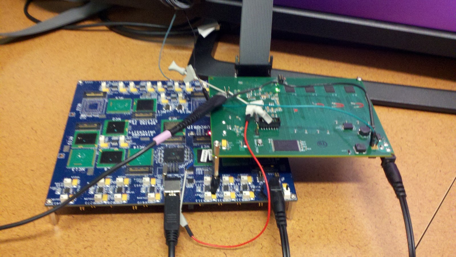
3. Connect as shown
1. Connect FPGA reset pin to Neurogrid reset
2. Connect FPGA acknowledge pin to oscilloscope and logic analyzer

Set up Logic Analyzer

1. load Stimulus\System1.tla configuration file
2. go to setup > probes tab
3. look for signals on channel 7
1. Probes C3 and C2 should be all triggering except first channel on C3
4. Start spring gui, and if software doesnt see sufficient signal, gui will time out.
1. The board light will trip.  This is normal for this experiment

Set up Software
In neuro-boa/apps/loopback_test/

1. Edit loopback_parameters.py
2. python loopback_parameters.py
3. python generate_spikes.py

Run experiment

1. In spring, run NEF/loopback_test/loopback_test.py
2. Right before experiment starts (when terminal shows "Update called to replace child:" , run logic analyzer
3. When logic analyzer stops, File > export data

Analyze data

1. Transfer logic analyzer data to desktop
2. Use loopback_test/ReadLAdataAllGroupsMultipleFilesStimulus.nb Mathematica script to parse logic analyzer data
1. change input file names
2. change output file names
3. Use loopback_test/cleanLogicData.sh to clean the spike data
1. change input file names
4. python loopback_test/analyze_loopback.py to analyze the spike data

Logic Analyzer Spike Time Cleanup Script

Here's a little bash script I use for cleaning up data files of spike times returned by the logic analyzer experiment

#!/bin/bash
# Cleans up logic analyzer data files prepended with "spike_times_"

FILES=spike_times_*

clean_file()
{
 echo processing $f
  sed -i 's/{//g' $1  # remove '{' at beginning of file
  sed -i 's/}//g' $1  # remove '}' at end of file
  sed -i 's/\ //g' $1  # remove ' ' spaces
  sed -i 's/,/\n/g' $1 # replace ',' with newlines
  sed -i '/^$/d' $1  # remove empty lines
}


for f in $FILES
do
 clean_file $f
done

DSP facts

Autocorrelation
in general:
\[
\phi_{yy}[n, n+m] = \text{E}\{y[n]y[n+m]\}
\]
if stationary
\[
\phi_{yy}[n, n+m] =  \phi_{yy}[m] = \text{E}\{\mathbf{y}_{n+m}\mathbf{y}_n^*\}
\]

Deterministic autocorrelation

\[
c_{hh}[l] = \sum_{k=-\infty}^{\infty}h[k]h[l+k] = h[n]*h[-n]
\]
\[
C_{hh}(e^{j\omega}) = H(e^{j\omega})H^*(e^{j\omega}) = |H(e^{j\omega})|^2
\]

Response of LTI system to random input
\[
\Phi_{yy}(e^{j\omega})=C_{hh}(e^{j\omega})\Phi_{xx}(e^{j\omega})
\]

Mean
$m_{\mathbf{x}_n}} = \text{E}\{\mathbf{x}_n\}$
if stationary $m_{\mathbf{x}_n}}=m_x \quad \text{for all } n$
Mean-squared (average power)
$\text{E}\{\mathbf{x}_n\mathbf{x}_n^*\} = \text{E}\{|\mathbf{x}_n|^2\} $
if stationary $\text{E}\{\mathbf{x}_n\mathbf{x}_n^*\} = \text{E}\{\mathbf{x}[n+m]\mathbf{x}[n]\}|_{m=0} = \phi_{xx}[0]$

Inverse DTFT
\[
x[n]=\frac{1}{2\pi} \int_{-\pi}^{\pi} X(e^{j\omega})e^{j\omega n}d\omega
\]
DTFT
\[
X(e^{j\omega}) = \sum_{n=-\infty}^{\infty}x[n]e^{j\omega n}
\]

Partial Derivative Logistic Regression Cost Function

Logistic regression is used for classification problems.  As Andrew said, it's a bit confusing given the "regression" in the name.

LR cost function is given by:
\[
\text{Cost} (h_\theta (x),y) =
\begin{cases}
 -\log(h_\theta (x)) \quad &\text{if } y=1 \\
 -\log(1-h_\theta (x)) \quad &\text{if } y=0
\end{cases}
\]

where \(h_\theta(x) = \frac{1}{1+e^{-\theta^Tx}}\) is the logistic function.

Since \(y \in \{0,1\}\) only, we can reduce the cost function to an equivalent, single equation.
\[
\text{Cost} (h_\theta (x),y) =  -y\log(h_\theta (x)) - (1-y)\log(1-h_\theta (x))
\]

This leads to the overall cost function for the logistic regression:
\[
J(\theta) = -\frac{1}{m} [\sum_{i=1}^m y^{(i)}\log h_\theta(x^{(i)}) + (1-y^{(i)})\log(1-h_\theta (x))]
\]

Our goal is to find \(\min_\theta J(\theta)\). To do so, we use gradient descent, but we first need to find the partial derivatives \(\frac{\partial}{\partial \theta_j} J(\theta)\).

We're going to make use of a neat property of the logistic function:
\begin{align}
g'(z) &= \frac{d}{dz} \frac{1}{1+e^{-z}} = \frac{1}{(1+e^{-z})^2}e^{-z} \\
 &= \frac{1+e^{-z}-1}{(1+e^{-z})^2} = \frac{1}{1+e^{-z}}-\frac{1}{(1+e^{-z})^2} = \frac{1}{1+e^{-z}}(1-\frac{1}{1+e^{-z}}) \\
 &= g(z) (1-g(z))
\end{align}

So for our with our cost function:
\begin{align}
\frac{\partial}{\partial \theta_j} J(\theta) &= -\frac{1}{m} \left [\frac{\partial}{\partial \theta_j} \sum_{i=1}^m y^{(i)}\log h_\theta(x^{(i)}) + (1-y^{(i)})\log(1-h_\theta (x)) \right] \\
 &= -\frac{1}{m} \left [ \sum_{i=1}^m y^{(i)}\frac{1}{h_\theta(x^{(i)})}\frac{\partial}{\partial \theta_j}h_\theta(x^{(i)}) + (1-y^{(i)})\frac{1}{1-h_\theta(x^{(i)})}\left (-\frac{\partial}{\partial \theta_j}h_\theta (x^{(i)})\right) \right]
\end{align}

using the chain rule and the logistic regression derivative, we see that
\begin{align}
\frac{\partial}{\partial \theta_j} J(\theta) &=-\frac{1}{m} \left [ \sum_{i=1}^m y^{(i)}\frac{x_j^{(i)}}{h_\theta(x^{(i)})}h_\theta(x^{(i)})(1-h_\theta(x^{(i)})) - (1-y^{(i)})\frac{x_j^{(i)}}{1-h_\theta(x^{(i)})}h_\theta (x)(1-h_\theta(x^{(i)})) \right] \\
&=  -\frac{1}{m} \left [ \sum_{i=1}^m y^{(i)}x_j^{(i)}(1-h_\theta(x^{(i)})) - (1-y^{(i)})x_j^{(i)}h_\theta (x^{(i)})) \right] \\
&=  -\frac{1}{m} \left [ \sum_{i=1}^m y^{(i)}x_j^{(i)} - x_jh_\theta (x^{(i)}) \right] \\
\frac{\partial}{\partial \theta_j} J(\theta) &=  \frac{1}{m} \sum_{i=1}^m  (h_\theta (x^{(i)}) -  y^{(i)}) x_j^{(i)}
\end{align}

This formula can now be used in gradient descent.

cleaning up unwanted data files from a git repository

I recently made the mistake of merging unwanted data files into the lab git repository, and unfortunately and these files weren't discovered until after they were also pushed to the remote repository.

To clean up the git repository, I used the git filter-branch command, force pushed the changes to the remote, and then had collaborators rebase their local copies of the contaminated branch.

Using git filter branch:

git filter-branch --index-filter 'git rm --cached --ignore-unmatch [filename]' --[commit to begin with]^..
rm -Rf .git/refs/original
rm -Rf .git/logs
git gc

Force pushing the changes:
git push --force origin [branch name]

Have collaborators rebase their local branches
git fetch (NOT PULL!!!!!)
git rebase --onto origin/[branch] [branch] [local branch ([branch] and anything derived from [branch])]

The last command does a hard reset on of the current branch to origin/[branch].  It then takes the commits from [local branch] and [branch] and then applies them to the current branch.

In addition I learned how to use regex to search for files matching wildcards through subdirectories -- you need to use the escape character \

e.g. to git remove all .txt files from a directory and all subdirectories:
git -rm ./\*.txt
without the escape character, the * wildcard is expanded by the shell.  with the escape character, git rm is allowed to interpret the *.txt

Connecting to wireless via command line

to initialize the interface: sudo ifconfig <interface name like wlan0> up
to connect to wireless: sudo iwconfig <interface name> essid <network name like Stanford>
to obtain an ipaddress: sudo dhclient <interface name>
to test whether connection is valid: ping -c 1 www.google.com

Adding a printer ubuntu

Problem is that nobody remembers the root password, which the system prompts you for upon selecting add printer in either the printers gui or localhost:631

The way around this was to run sudo system-config-printer from the command line...

Synapse Calibration procedure

on ng-thalamu

There are 4 steps to the calibration:

1. gleak
2. Erev
3. txmt
4. tau_lpf

For gleak (Erev)

1. Arrange the board's xml file so the chip and synapse numbers you are looking to calibrate are first in the file
2. Match the chip and synapse numbers in syn_f_vs_g_sleak.py (f_vs_erev_sleak.py) to the desired chip and synapse numbers AND BE SURE TO SAVE.
3. In spring, run  syn_f_vs_g_sleak.py (f_vs_erev_sleak.py)
4. Set the chip and synapse numbers in calib_syn_f_vs_g_sleak.py (calib_f_vs_erev_sleak.py) to the desired chip and synapse numbers AND BE SURE TO SAVE.
5. Run calib_syn_f_vs_g_sleak.py (calib_f_vs_erev_sleak.py) in ipython --pylab
6. Execute extract_syn_param_g_lksoma.py (extract_syn_param_erev_lksoma.py) in ipython --pylab, and then call run_default with the appropriate bif file, board name, chip number, and synapse number.
7. Use median values in histogram as parameters in xml file

For txmt (tau_lpf)

1. In neuro-boa/apps/calibrate_neuron/calibrate_synapse/calibrate_pe/calibrate_pe.cpp (calibrate_vleakpf/calibrate_vleakpf.cpp):
1.  make sure the appropriate chip calibration is pushed back
• CALIBRATION_DAC_FILE.push_back(<check this>);
• CALIBRATION_ADC_FILE.push_back(<check this>);
2. make sure the appropriate chip number is pushed back
• selected_chips.push_back(<chip number>);
3. select the appropriate chip in the for loop around ~line 621
2. run make
3. run calibrate_pe (calibrate_vleakpf)
4. For txmt:
1. change pw_values.csv to pw_values_<board>_<chip>.csv
2. In fit_2d_1coeff.py
• change filename to match data
• select synapse
3. run fit_2d_1coeff.py
4. set C1 to median value
5. set C3 to 0
5. For tau_lpf:
1. change the data/ folder name to data<chip num>/
2. In fit_tau.py
1. change data folder to match chip number
3. run fit_tau.py
4. set tau_lpf to median value

Synaptic Pulse extender

On Neurogrid, the synaptic conductance, \(x\), is governed by
\[\tau \dot{x} = -x + g_{max}\sum_ip(t-t_i)\]
where \(p(t)\) is a square pulse of length \(t_{xmt}\) resulting from spikes arriving at time \(t_i\), \(g_{max}\) is the maximum synaptic conductance, and \(\tau\) is the synaptic time constant.

Let's analyze the steady state conductance induced by a Poisson spike train where the interarrival times of spikes are distributed exponentially with pdf \(f(t) = \lambda e^{-\lambda t}\).

At steady state, \(\dot{x} = 0\), and \(0 = -x + g_{max}p(t)\).
Therefore at steady state, \(x = g_{max}p(t)\) and on average \(\langle x \rangle=g_{max} \langle p(t) \rangle\).

There is one wrinkle in our analysis: when a spike arrives within \(t_{xmt}\) of the previous spike. The two resulting pulses do not add linearly.  The second pulse merely extends the previous pulse by the time between the spikes.

\[\langle p(t)\rangle=\langle \mathrm{spike\ rate}\rangle \langle \mathrm{average\ pulse\ value}\rangle\]

For a Poisson process, the rate is simply \(\lambda\).

For a full pulse, the area is simply \(t_{xmt}\).  For the pulse resulting from a collision, the area is \(t=\Delta t\). So

\[\langle \mathrm{average\ pulse\ value}\rangle = \int_0^{t_{xmt}} t \lambda e^{-\lambda t} dt + \int_{t_{xmt}}^\infty t_{xmt}\lambda e^{-\lambda t} dt\]

\[ = \left. t e^{-\lambda t}\right|_{t_{xmt}}^0 + \int_0^{t_{xmt}} e^{-\lambda t} dt + \left. t_{xmt}\lambda e^{-\lambda t} \right|_\infty^{t_{xmt}}\]
\[ = -t_{xmt} e^{-\lambda t_{xmt}} + \left. \frac{1}{\lambda} e^{-\lambda t} \right|_{t_{xmt}}^0 + t_{xmt}\lambda e^{-\lambda t_{xmt}} \]

\[ = \frac{1}{\lambda} (1-e^{-\lambda t_{xmt}})\]

\[\langle p(t)\rangle = \lambda \frac{1}{\lambda} (1-e^{-\lambda t_{xmt}})\]
\[\langle p(t)\rangle = (1-e^{-\lambda t_{xmt}})\]

The average synaptic conductance is then
\[\langle x \rangle = g_{max}(1-e^{-\lambda t_{xmt}})\]

Useful Laplace techniques

Final Value Theorem:
$\lim_{x \to \infty} x(t) = \lim_{s \to 0} sX(s)$
don't forget about the extra $s$ in the rhs.

Linear Systems and DiffEqs

I came across the most wonderful diagram on Richard Prager's Cambridge engineering mathematics course site relating differential equations to linear systems analysis. If only I had see this when I was taking signals and systems!  
differential equation --> solve --> compute step response --> differentiate --> voila! you have the impulse response and can now calculate the response to any input.

I've been having trouble focusing recently.  I think it's because I have lab presentation in a couple of weeks but I feel like I have little results to share with the group.
There is hope though.  I should talk to Nick about his synaptic gain modulation again and see what conclusions we drew from his presentation.

Things I can present:
Kalman filter update (ie integrator update)
Synaptic gain modulation
-does QIF neuron support it
Robot plan
-simulation results would be great

Remote desktop with x11 vnc

x11 vnc allows for remote desktop access

It's a simple system to use:

• ssh into the computer you would like to remotely access.
• run x11vnc on the remote computer
• it should print out something like: "The VNC desktop is:      <remote_host>:<display number>
• on your local computer, run vncviewer <remote_host>:<display number>

This guy developed x11vnc.

Setting up user accounts on ubuntu

Creating an account:
useradd -m <username>

Don't forget the -m!!!!! or they won't have a home folder and hence desktop and it will be very confusing!

Change shell to bash
chsh -s /bin/bash <username>

Man, there are so many little details under the hood of Ubuntu that you can miss! Yes, it gives you a lot of control, but the learning curve is super steep!

Linearization

Linearization is the idea of approximating a continuous function around a point with a line.
For a continuous function \(f(x)\), we linearize \(f(x)\) around point \(a\) as
\[f(x)\approx f(a) + f'(a)(x-a).\]

More interesting things happen in higher dimensions:
\[f(\mathbf{x}) \approx f(\mathbf{a}) + \left. \frac{\partial f(\mathbf{x})}{\partial x_1}\right|_{\mathbf{a}} + \left. \frac{\partial f(\mathbf{x})}{\partial x_2}\right|_{\mathbf{a}} + \ldots \]
or
\[f(\mathbf{x}) \approx f(\mathbf{a}) + \left. \nabla f \right|_{\mathbf{a}}  \cdot ({\mathbf{x}} - {\mathbf{a}}) .\]

You My Friend

My Russian coworker explained to me why Russians say You my friend".
English sentences have subjects and verbs.
"You are my friend"
subject: you
verb: are

But here, the words "you" and "are" are redundant.  In Russian, these two words would simply be lumped together into "you", so "you are my friend" becomes (with thick accent) "you my friend".