Notes from CS 222 - Differential Equations in Action

In units 1 and 2, we worked towards simulating Apollo 13's flight from the earth, around the moon, and back to earth. 

$h$ - step size

$x$ - position

$v$ - velocity

$F$ - net force 

$m$ - mass

Euler's method:

Euler's method is the most basic and easy to understand method for simulating a differential equation.  At each step in time, we simply increment the state variables linearly along the line tangent to their current values.

$x[i + 1] = x[i] + h \cdot v[i]$

$v[i + 1] = v[i] + h \cdot \frac{F(x[i],v[i])}{m}$

In the limiting case where $h\to0$, Euler's method will capture the dynamics exactly, but this makes the method very computationally intensive.  Values of $h>0$ will all lead to a certain amount of error at each step, known as the Local Truncation Error.

Heun's method

Heun's method is an improvement on Euler's method.  Rather than increment along the line tangent to the state variables, we use the average of the lines tangent to the state variable at the current point and the tangent to the state variable at the next point had we used Euler's method.

$x_E = x[i] + h \cdot v[i]$

$v_E = v[i] + h \cdot \frac{F(x[i],v[i])}{m}$

$x[i + 1] = x[i] + h \cdot \frac{v[i] + v_E}{2}$

$v[i + 1] = v[i] + h \cdot \frac{F(x[i], v[i]) + F(x_E, v_E)}{2m}$

where $x_E$ and $v_E$ are simply the Euler estimates of the next $x$ and $v$

Adaptive step size

[Needs work]

$h_{new} = h_{old}\sqrt{\frac{tolerance}{LTE}}$

Note that you'll need to track the current time with this method since our time steps will not be evenly spaced.

Simplectic method

[Needs work]

A plot of the state variables is called a phase space plot.  The area of the phase space plot is the energy? of the system. The simplectic method preserves the energy of the system.  In the simplectic method, we alternate between incrementing state variables.

$x[i + 1] = x[i] + h \cdot v[i]$

$v[i + 1] = v[i] + h \cdot \frac{F(x[i+1], v[i])}{m}$

There are a few alternatives to this:

•  $x$ then $v$ then $v$ then $x$ ... etc. This is known as leapfrogging

Visiting Penelope at 6 months

Penelope "Pom Pom" is my niece!

Successful diaper change. Penelope is really happy when you lift her up like this.

Here are some vignettes from my visit:

Pom Pom had a cold during my visit.  It's really a terrible thing to have a cold as an infant.  You don't even know to how wipe your nose! In fact, rather than wipe your nose after sneezing out a bunch of mucus, you'd rather open your mouth for a taste.  Truly a curious being.
This leaves it to the nearest adult to wipe your nose for you.  However, Pom Pom is a free willed spirit.  She could be smiling happily with snot all over her face one second, but the moment you touch her face with a kleenax to wipe it off, insanity follows.  Head turns away, back arches, arms reach out, legs kick away, and Pom Pom screams.  Every muscle she can control is activated to escape that terrible terrible kleenax.  Pom Pom has her own designs for cleaning her face. If you hold her on your shoulder, her trick is to happy to bury her runny face in the crook of your shoulder and then wipe all that wonderful juice in the perfect arc across your shirt.
The solution: put a kleenax on your shoulder.

PP is learning to crawl. Not deliberately, of course. I doubt babies so purposely and single-mindedly pursue activities like an adult will try to say learn to swim.  PP is motivated by the toy or computer immediately in front of her, and she'll try anything she can to move towards the object of her motivation.  When PP tries to move forward, she pushes out with her hands and legs. Only her hands gain traction though and she ends up pushing herself backwards.

Babies have no memories.  How can the PP be entertained by a toy for 20 min, get bored, then be returned an hour later and be entertained by the same toy for another 20 min!

Flow for Logic Analyzer Experiment

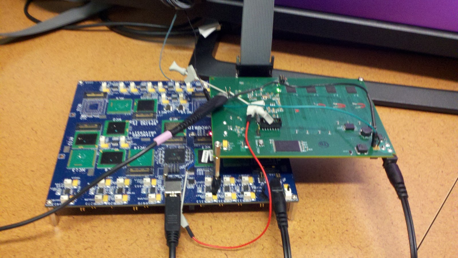
To root out the causes of time dilation, I've set up a flow for collecting spike time stamps from Neurogrid for comparing them with the programmed spike times.  I can then compare the measured ISIs (to the tens of picosecond resolution) to the programmed ISIs.  Time dilation manifests as an additional delay in the ISI, and likewise time contraction manifests as a shortening of the ISI.

Flow:

Set up Neurogrid

1. Connect FPGA to leaf of 9
2. Spoof FPGA as chip 15
1. change xml config file so 15 is at leaf of 9
2. comment out chip 17 in xml config file route (17 is normal FPGA)
3.  In bias-ZIF-6k.xml, change chip_15 route_to to match xml config file 
3. Connect as shown
1. Connect FPGA reset pin to Neurogrid reset
2. Connect FPGA acknowledge pin to oscilloscope and logic analyzer

Set up Logic Analyzer

1. load Stimulus\System1.tla configuration file
2. go to setup > probes tab
3. look for signals on channel 7
1. Probes C3 and C2 should be all triggering except first channel on C3
4. Start spring gui, and if software doesnt see sufficient signal, gui will time out.
1. The board light will trip.  This is normal for this experiment

Set up Software
In neuro-boa/apps/loopback_test/

1. Edit loopback_parameters.py
2. python loopback_parameters.py
3. python generate_spikes.py

Run experiment

1. In spring, run NEF/loopback_test/loopback_test.py
2. Right before experiment starts (when terminal shows "Update called to replace child:" , run logic analyzer
3. When logic analyzer stops, File > export data

Analyze data

1. Transfer logic analyzer data to desktop
2. Use loopback_test/ReadLAdataAllGroupsMultipleFilesStimulus.nb Mathematica script to parse logic analyzer data
1. change input file names
2. change output file names
3. Use loopback_test/cleanLogicData.sh to clean the spike data
1. change input file names
4. python loopback_test/analyze_loopback.py to analyze the spike data

Logic Analyzer Spike Time Cleanup Script

Here's a little bash script I use for cleaning up data files of spike times returned by the logic analyzer experiment

#!/bin/bash
# Cleans up logic analyzer data files prepended with "spike_times_"

FILES=spike_times_*

clean_file()
{
 echo processing $f
  sed -i 's/{//g' $1  # remove '{' at beginning of file
  sed -i 's/}//g' $1  # remove '}' at end of file
  sed -i 's/\ //g' $1  # remove ' ' spaces
  sed -i 's/,/\n/g' $1 # replace ',' with newlines
  sed -i '/^$/d' $1  # remove empty lines
}


for f in $FILES
do
 clean_file $f
done

DSP facts

Autocorrelation
in general:
\[
\phi_{yy}[n, n+m] = \text{E}\{y[n]y[n+m]\}
\]
if stationary
\[
\phi_{yy}[n, n+m] =  \phi_{yy}[m] = \text{E}\{\mathbf{y}_{n+m}\mathbf{y}_n^*\}
\]

Deterministic autocorrelation

\[
c_{hh}[l] = \sum_{k=-\infty}^{\infty}h[k]h[l+k] = h[n]*h[-n]
\]
\[
C_{hh}(e^{j\omega}) = H(e^{j\omega})H^*(e^{j\omega}) = |H(e^{j\omega})|^2
\]

Response of LTI system to random input
\[
\Phi_{yy}(e^{j\omega})=C_{hh}(e^{j\omega})\Phi_{xx}(e^{j\omega})
\]

Mean
$m_{\mathbf{x}_n}} = \text{E}\{\mathbf{x}_n\}$
if stationary $m_{\mathbf{x}_n}}=m_x \quad \text{for all } n$
Mean-squared (average power)
$\text{E}\{\mathbf{x}_n\mathbf{x}_n^*\} = \text{E}\{|\mathbf{x}_n|^2\} $
if stationary $\text{E}\{\mathbf{x}_n\mathbf{x}_n^*\} = \text{E}\{\mathbf{x}[n+m]\mathbf{x}[n]\}|_{m=0} = \phi_{xx}[0]$

Inverse DTFT
\[
x[n]=\frac{1}{2\pi} \int_{-\pi}^{\pi} X(e^{j\omega})e^{j\omega n}d\omega
\]
DTFT
\[
X(e^{j\omega}) = \sum_{n=-\infty}^{\infty}x[n]e^{j\omega n}
\]

Partial Derivative Logistic Regression Cost Function

Logistic regression is used for classification problems.  As Andrew said, it's a bit confusing given the "regression" in the name.

LR cost function is given by:
\[
\text{Cost} (h_\theta (x),y) =
\begin{cases}
 -\log(h_\theta (x)) \quad &\text{if } y=1 \\
 -\log(1-h_\theta (x)) \quad &\text{if } y=0
\end{cases}
\]

where \(h_\theta(x) = \frac{1}{1+e^{-\theta^Tx}}\) is the logistic function.

Since \(y \in \{0,1\}\) only, we can reduce the cost function to an equivalent, single equation.
\[
\text{Cost} (h_\theta (x),y) =  -y\log(h_\theta (x)) - (1-y)\log(1-h_\theta (x))
\]

This leads to the overall cost function for the logistic regression:
\[
J(\theta) = -\frac{1}{m} [\sum_{i=1}^m y^{(i)}\log h_\theta(x^{(i)}) + (1-y^{(i)})\log(1-h_\theta (x))]
\]

Our goal is to find \(\min_\theta J(\theta)\). To do so, we use gradient descent, but we first need to find the partial derivatives \(\frac{\partial}{\partial \theta_j} J(\theta)\).

We're going to make use of a neat property of the logistic function:
\begin{align}
g'(z) &= \frac{d}{dz} \frac{1}{1+e^{-z}} = \frac{1}{(1+e^{-z})^2}e^{-z} \\
 &= \frac{1+e^{-z}-1}{(1+e^{-z})^2} = \frac{1}{1+e^{-z}}-\frac{1}{(1+e^{-z})^2} = \frac{1}{1+e^{-z}}(1-\frac{1}{1+e^{-z}}) \\
 &= g(z) (1-g(z))
\end{align}

So for our with our cost function:
\begin{align}
\frac{\partial}{\partial \theta_j} J(\theta) &= -\frac{1}{m} \left [\frac{\partial}{\partial \theta_j} \sum_{i=1}^m y^{(i)}\log h_\theta(x^{(i)}) + (1-y^{(i)})\log(1-h_\theta (x)) \right] \\
 &= -\frac{1}{m} \left [ \sum_{i=1}^m y^{(i)}\frac{1}{h_\theta(x^{(i)})}\frac{\partial}{\partial \theta_j}h_\theta(x^{(i)}) + (1-y^{(i)})\frac{1}{1-h_\theta(x^{(i)})}\left (-\frac{\partial}{\partial \theta_j}h_\theta (x^{(i)})\right) \right]
\end{align}

using the chain rule and the logistic regression derivative, we see that
\begin{align}
\frac{\partial}{\partial \theta_j} J(\theta) &=-\frac{1}{m} \left [ \sum_{i=1}^m y^{(i)}\frac{x_j^{(i)}}{h_\theta(x^{(i)})}h_\theta(x^{(i)})(1-h_\theta(x^{(i)})) - (1-y^{(i)})\frac{x_j^{(i)}}{1-h_\theta(x^{(i)})}h_\theta (x)(1-h_\theta(x^{(i)})) \right] \\
&=  -\frac{1}{m} \left [ \sum_{i=1}^m y^{(i)}x_j^{(i)}(1-h_\theta(x^{(i)})) - (1-y^{(i)})x_j^{(i)}h_\theta (x^{(i)})) \right] \\
&=  -\frac{1}{m} \left [ \sum_{i=1}^m y^{(i)}x_j^{(i)} - x_jh_\theta (x^{(i)}) \right] \\
\frac{\partial}{\partial \theta_j} J(\theta) &=  \frac{1}{m} \sum_{i=1}^m  (h_\theta (x^{(i)}) -  y^{(i)}) x_j^{(i)}
\end{align}

This formula can now be used in gradient descent.

cleaning up unwanted data files from a git repository

I recently made the mistake of merging unwanted data files into the lab git repository, and unfortunately and these files weren't discovered until after they were also pushed to the remote repository.

To clean up the git repository, I used the git filter-branch command, force pushed the changes to the remote, and then had collaborators rebase their local copies of the contaminated branch.

Using git filter branch:

git filter-branch --index-filter 'git rm --cached --ignore-unmatch [filename]' --[commit to begin with]^..
rm -Rf .git/refs/original
rm -Rf .git/logs
git gc

Force pushing the changes:
git push --force origin [branch name]

Have collaborators rebase their local branches
git fetch (NOT PULL!!!!!)
git rebase --onto origin/[branch] [branch] [local branch ([branch] and anything derived from [branch])]

The last command does a hard reset on of the current branch to origin/[branch].  It then takes the commits from [local branch] and [branch] and then applies them to the current branch.

In addition I learned how to use regex to search for files matching wildcards through subdirectories -- you need to use the escape character \

e.g. to git remove all .txt files from a directory and all subdirectories:
git -rm ./\*.txt
without the escape character, the * wildcard is expanded by the shell.  with the escape character, git rm is allowed to interpret the *.txt